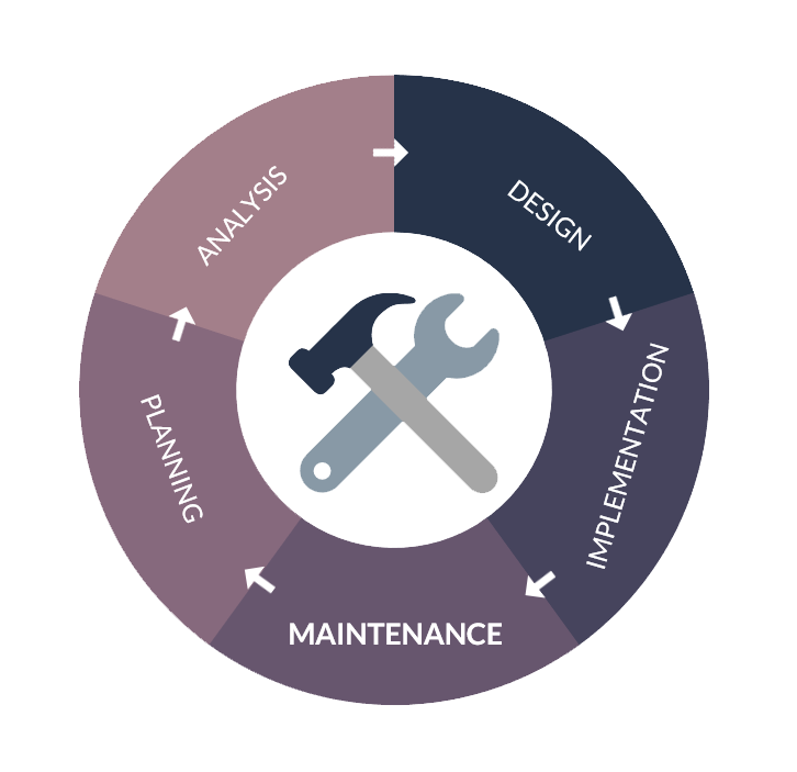
In the last article, we promised to present the process of implementing predictive maintenance using Artificial Intelligence. And that’s exactly what we are going to do! Although the process will vary in each case there are certain steps that need to be followed every time.
It’s important to note that this process is an on-going cycle, and that means each phase may have to be revised if the results of the entire cycle are unsatisfactory.

Phase 1: Collecting and analyzing data
Precise analysis requires adequate data. Different equipment and machines require different sensors for us to monitor their technical conditions. Data that we gather provides insights and draws correlations between values and the equipment’s actual state. We need to monitor and notice abnormalities before a malfunction occurs.
In the next step, we need to find the most efficient set of features for our model. Irrelevant features would decrease the model’s accuracy because it would learn from useless data. Once we select the right features, we have to filter out data’s “noise”.
It’s important for us to select the right attributes to avoid obviously incorrect sensor indications. For example, when we measure temperatures from a sensor, a result of -200 degrees Celsius is obviously incorrect and we should ignore it. We have to prepare the data in a way that allows for use in a machine learning model, meaning the data must be properly formatted. The network requires input data (requests) and output data (feedback) and we must filter out the incomplete results.
The last thing we have left to do is dividing the data into 2 groups: training and testing data. The same datasets cannot be used for both training and evaluating otherwise the AI would learn the correct answers and “cheat”.
Phase 2: Creating the prediction model and its development
With the data processed enough for Artificial Intelligence algorithms to use, it’s time to choose the right deep learning model. Using the features that we picked earlier, we will try to find the most accurate model possible. There’s a wide variety of criteria, but for the maintenance purposes measuring methods that penalize significant errors are necessary. Root mean squared deviation will force the forecast Remaining Useful Life (RUL) as close as possible.
With the model tested, tweaked and ready, it’s time to develop the real-life solution for the production.
What’s next?
The next phase is to develop a real-life solution for production. This step will be covered thoroughly in the next article of this mini-series. To stay up to date, follow us on Linkedin!


